Demo: Steady Multiphysics Simulation (Coupled Diffusion Reaction)
This demo code demonstrate how to solve a steady coupled Advection-Diffusion-Reaction problem with surface reaction terms at the boundary. This demo is used to demonstrate how to use the MultiphysicsProblem class in FLATiron.
The source code can be found in demo/demo_steady_multiphysics/demo_steady_multiphysics.py.
Problem definition
First we define the concentration of chemical species \(A\), \(B\), and \(C\), for a 1D domain of length \(L\), we have
The left boundary conditions are as follows
And the surface reactions on the right boundary
Implementation
Fist, we import code the relevant modules from flatiron_tk and the basic libraries and define the mesh and constants.
import dolfinx
import ufl

from flatiron_tk.mesh import RectMesh
from flatiron_tk.physics import MultiphysicsProblem
from flatiron_tk.physics import SteadyScalarTransport
from flatiron_tk.solver import NonLinearProblem
from flatiron_tk.solver import NonLinearSolver


'''
Demo for a coupled diffusion reaction problem
D_A \\frac{d^2A}{dx^2} - k_v A B = 0
D_B \\frac{d^2B}{dx^2} - 2k_v A B = 0
D_C \\frac{d^2C}{dx^2} + k_v A B = 0

BC:
A(x=0) = C0
B(x=0) = C0
C(x=0) = 0

\\nabla A \\cdot \\hat{n} = -k_S A B  / D_A \\forall \\vec{x} \\in \\Gamma_B
\\nabla B \\cdot \\hat{n} = -2K_S A B / D_B \\forall \\vec{x} \\in \\Gamma_B
\\nabla C \\cdot \\hat{n} = K_s A B   / D_C \\forall \\vec{x} \\in \\Gamma_B
'''

# Create Mesh
mesh = RectMesh(0.0, 0.0, 4.0, 1.0, 1/64)

# Define Constants
D_A = 0.1; D_B = 0.1; D_C = 0.1
k_v = dolfinx.fem.Constant(mesh.msh, dolfinx.default_scalar_type(0.01))
k_s = 1
c0 = 1
u_mag = 10.0

# Create the velocity field
U = u_mag
x = ufl.SpatialCoordinate(mesh.msh)
u = ufl.as_vector([U * x[1] * (1 - x[1]), 0.0])
Next we define SteadyScalarTransport problems for all three species and set the appropriate tag to disambiguate them.
# Define Physics A, B, C
stp_A = SteadyScalarTransport(mesh, tag='A', q_degree=5)
stp_A.set_element('CG', 1)
stp_A.set_advection_velocity(u)
stp_A.set_diffusivity(D_A)

stp_B = SteadyScalarTransport(mesh, tag='B', q_degree=5)
stp_B.set_element('CG', 1)
stp_B.set_advection_velocity(u)
stp_B.set_diffusivity(D_B)

stp_C = SteadyScalarTransport(mesh, tag='C', q_degree=5)
stp_C.set_element('CG', 1)
stp_C.set_advection_velocity(u)
stp_C.set_diffusivity(D_C)
Now we build a MultiPhysicsProblem as a collection of the three ScalarTransport physics that we created.
# Build Multiphysics Problem
coupled_physics = MultiphysicsProblem(stp_A, stp_B, stp_C)
coupled_physics.set_element()
coupled_physics.build_function_space()
Now, we will set the terms which couple the three equations together. This is done by first grabbing the solution
function of from each species through the get_solution_function() method by supplying the appropriate tag for each species.
Then we set reaction associated with each species’ equation through the set_reaction() function on the
individual SteadyScalarTransport object. Finally, we finalize the volumetric weak formulation. We additionally add
SUPG stabilization to each equation.
A = coupled_physics.get_solution_function('A')
B = coupled_physics.get_solution_function('B')
C = coupled_physics.get_solution_function('C')

stp_A.set_reaction(-k_v * A * B)
stp_B.set_reaction(-2 * k_v * A * B)
stp_C.set_reaction(k_v * A * B)

# Set weak form and stabilization
stp_options = {'stab':True}
coupled_physics.set_weak_form(stp_options,stp_options,stp_options)
Now we set the boundary conditions dictionary for each physics and create an overall dictionary with the species tag
called bc_dict which we supply into the coupled_physics object. The format for the individual boundary condition dictionary
has the same format as a single species transport problem. Here, we utilize the solution functions that we
grabbed earlier to define the Neumann boundary condition. We can do this because Neumann boundary condition is
simply an additional term in the weak formulation.
# 5 = left,
# 8 = bottom
n = mesh.get_facet_normal()
A_bcs = {
    1: {'type': 'dirichlet', 'value': dolfinx.fem.Constant(mesh.msh, dolfinx.default_scalar_type(c0))},
    2: {'type': 'neumann', 'value': -k_s*A*B/D_A * n}
}
B_bcs = {
    1: {'type': 'dirichlet', 'value': dolfinx.fem.Constant(mesh.msh, dolfinx.default_scalar_type(c0))},
    2: {'type': 'neumann', 'value': -2*k_s*A*B/D_B * n}
}
C_bcs = {
    1: {'type': 'dirichlet', 'value': dolfinx.fem.Constant(mesh.msh, dolfinx.default_scalar_type(0.0))},
    2: {'type': 'neumann', 'value': k_s*A*B/D_C * n}
}

bc_dict = {
    'A': A_bcs,
    'B': B_bcs,
    'C': C_bcs
}

coupled_physics.set_bcs(bc_dict)
Finally, we create a nonlinear problem and solver to solve the coupled system.
# Set writers
coupled_physics.set_writer('output', 'pvd')

# Set problem
problem = NonLinearProblem(coupled_physics)
solver = NonLinearSolver(mesh.msh.comm, problem)

# Solve and write
solver.solve()
coupled_physics.write()
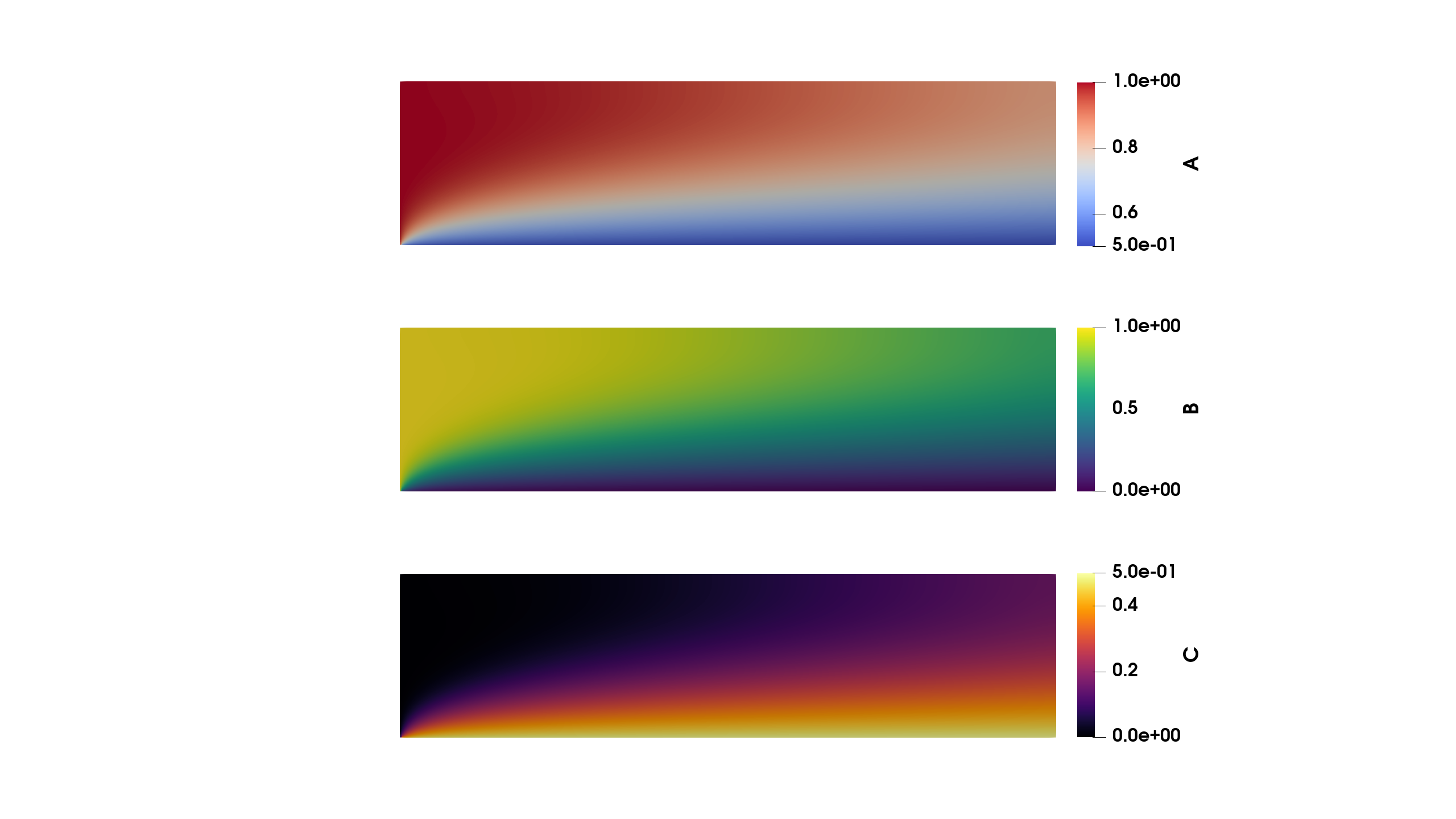
This code should give the following result:
Full Script
import dolfinx
import ufl

from flatiron_tk.mesh import RectMesh
from flatiron_tk.physics import MultiphysicsProblem
from flatiron_tk.physics import SteadyScalarTransport
from flatiron_tk.solver import NonLinearProblem
from flatiron_tk.solver import NonLinearSolver


'''
Demo for a coupled diffusion reaction problem
D_A \\frac{d^2A}{dx^2} - k_v A B = 0
D_B \\frac{d^2B}{dx^2} - 2k_v A B = 0
D_C \\frac{d^2C}{dx^2} + k_v A B = 0

BC:
A(x=0) = C0
B(x=0) = C0
C(x=0) = 0

\\nabla A \\cdot \\hat{n} = -k_S A B  / D_A \\forall \\vec{x} \\in \\Gamma_B
\\nabla B \\cdot \\hat{n} = -2K_S A B / D_B \\forall \\vec{x} \\in \\Gamma_B
\\nabla C \\cdot \\hat{n} = K_s A B   / D_C \\forall \\vec{x} \\in \\Gamma_B
'''

# Create Mesh
mesh = RectMesh(0.0, 0.0, 4.0, 1.0, 1/64)

# Define Constants
D_A = 0.1; D_B = 0.1; D_C = 0.1
k_v = dolfinx.fem.Constant(mesh.msh, dolfinx.default_scalar_type(0.01))
k_s = 1
c0 = 1
u_mag = 10.0

# Create the velocity field
U = u_mag
x = ufl.SpatialCoordinate(mesh.msh)
u = ufl.as_vector([U * x[1] * (1 - x[1]), 0.0])

# Define Physics A, B, C
stp_A = SteadyScalarTransport(mesh, tag='A', q_degree=5)
stp_A.set_element('CG', 1)
stp_A.set_advection_velocity(u)
stp_A.set_diffusivity(D_A)

stp_B = SteadyScalarTransport(mesh, tag='B', q_degree=5)
stp_B.set_element('CG', 1)
stp_B.set_advection_velocity(u)
stp_B.set_diffusivity(D_B)

stp_C = SteadyScalarTransport(mesh, tag='C', q_degree=5)
stp_C.set_element('CG', 1)
stp_C.set_advection_velocity(u)
stp_C.set_diffusivity(D_C)

# Build Multiphysics Problem
coupled_physics = MultiphysicsProblem(stp_A, stp_B, stp_C)
coupled_physics.set_element()
coupled_physics.build_function_space()

A = coupled_physics.get_solution_function('A')
B = coupled_physics.get_solution_function('B')
C = coupled_physics.get_solution_function('C')

stp_A.set_reaction(-k_v * A * B)
stp_B.set_reaction(-2 * k_v * A * B)
stp_C.set_reaction(k_v * A * B)

# Set weak form and stabilization
stp_options = {'stab':True}
coupled_physics.set_weak_form(stp_options,stp_options,stp_options)

# 5 = left,
# 8 = bottom
n = mesh.get_facet_normal()
A_bcs = {
    1: {'type': 'dirichlet', 'value': dolfinx.fem.Constant(mesh.msh, dolfinx.default_scalar_type(c0))},
    2: {'type': 'neumann', 'value': -k_s*A*B/D_A * n}
}
B_bcs = {
    1: {'type': 'dirichlet', 'value': dolfinx.fem.Constant(mesh.msh, dolfinx.default_scalar_type(c0))},
    2: {'type': 'neumann', 'value': -2*k_s*A*B/D_B * n}
}
C_bcs = {
    1: {'type': 'dirichlet', 'value': dolfinx.fem.Constant(mesh.msh, dolfinx.default_scalar_type(0.0))},
    2: {'type': 'neumann', 'value': k_s*A*B/D_C * n}
}

bc_dict = {
    'A': A_bcs,
    'B': B_bcs,
    'C': C_bcs
}

coupled_physics.set_bcs(bc_dict)

# Set writers
coupled_physics.set_writer('output', 'pvd')

# Set problem
problem = NonLinearProblem(coupled_physics)
solver = NonLinearSolver(mesh.msh.comm, problem)

# Solve and write
solver.solve()
coupled_physics.write()